VLFeat includes fast SVM solvers, SGC [1] and (S)DCA [2], both implemented in vl_svmtrain. The function also implements features, like Homogeneous kernel map expansion and SVM online statistics. (S)DCA can also be used with different loss functions.

Support vector machine

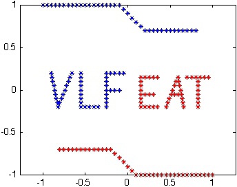
A simple example on how to use vl_svmtrain is presented below. Let's first load and plot the training data:

% Load training data X and their labels y
vl_setup demo % to load the demo data
load('vl_demo_svm_data.mat');

Xp = X(:,y==1);
Xn = X(:,y==-1);

figure
plot(Xn(1,:),Xn(2,:),'*r')
hold on
plot(Xp(1,:),Xp(2,:),'*b')
axis equal ;

Now we have a plot of the tutorial training data:

Training Data.

Now we will set the learning parameters:

lambda = 0.01 ; % Regularization parameter
maxIter = 1000 ; % Maximum number of iterations

Learning a linear classifier can be easily done with the following 1 line of code:

[w b info] = vl_svmtrain(X, y, lambda, 'MaxNumIterations', maxIter)

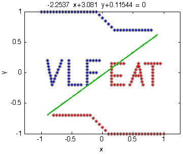
Now we can plot the output model over the training data.

% Visualisation
eq = [num2str(w(1)) '*x+' num2str(w(2)) '*y+' num2str(b)];
line = ezplot(eq, [-0.9 0.9 -0.9 0.9]);
set(line, 'Color', [0 0.8 0],'linewidth', 2);

The result is plotted in the following figure.

Learned model.

The output info is a struct containing some statistic on the learned SVM:

info =

            solver: 'sdca'
            lambda: 0.0100
    biasMultiplier: 1
              bias: 0.0657
         objective: 0.2105
       regularizer: 0.0726
              loss: 0.1379
     dualObjective: 0.2016
          dualLoss: 0.2742
        dualityGap: 0.0088
         iteration: 525
             epoch: 3
       elapsedTime: 0.0300

It is also possible to use under some assumptions [3] a homogeneous kernel map expanded online inside the solver. This can be done with the following commands:

% create a structure with kernel map parameters
hom.kernel = 'KChi2';
hom.order = 2;
% create the dataset structure
dataset = vl_svmdataset(X, 'homkermap', hom);
% learn the SVM with online kernel map expansion using the dataset structure
[w b info] = vl_svmtrain(dataset, y, lambda, 'MaxNumIterations', maxIter)

The above code creates a training set without applying any homogeneous kernel map to the data. When the solver is called it will expand each data point with a Chi Squared kernel of period 2.

Diagnostics

VLFeat allows to get statistics during the training process. It is sufficient to pass a function handle to the solver. The function will be then called every DiagnosticFrequency time.

(S)DCA diagnostics also provides the duality gap value (the difference between primal and dual energy), which is the upper bound of the primal task sub-optimality.

% Diagnostic function
function diagnostics(svm)
  energy = [energy [svm.objective ; svm.dualObjective ; svm.dualityGap ] ] ;
end

% Training the SVM
energy = [] ;
[w b info] = vl_svmtrain(X, y, lambda,...
                           'MaxNumIterations',maxIter,...
                           'DiagnosticFunction',@diagnostics,...
                           'DiagnosticFrequency',1)

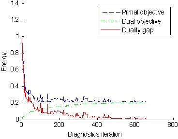
The objective values for the past iterations are kept in the matrix energy. Now we can plot the objective values from the learning process.

figure
hold on
plot(energy(1,:),'--b') ;
plot(energy(2,:),'-.g') ;
plot(energy(3,:),'r') ;
legend('Primal objective','Dual objective','Duality gap')
xlabel('Diagnostics iteration')
ylabel('Energy')

SVM objective values plot.

References

[1] Y. Singer and N. Srebro. Pegasos: Primal estimated sub-gradient solver for SVM. In Proc. ICML, 2007.
[2] S. Shalev-Schwartz and T. Zhang. Stochastic Dual Coordinate Ascent Methods for Regularized Loss Minimization. 2013.
[3] A. Vedaldi and A. Zisserman. Efficient additive kernels via explicit feature maps. In PAMI, 2011.

VLFeat.org

Table of Contents

Support vector machine

Diagnostics

References